Hub susceptibility
This page contains descriptions and examples to build hub susceptibility models. For additional details on hub susceptibility models, please see our manuscript entitled Network-based atrophy modeling in the common epilepsies: a worldwide ENIGMA study.
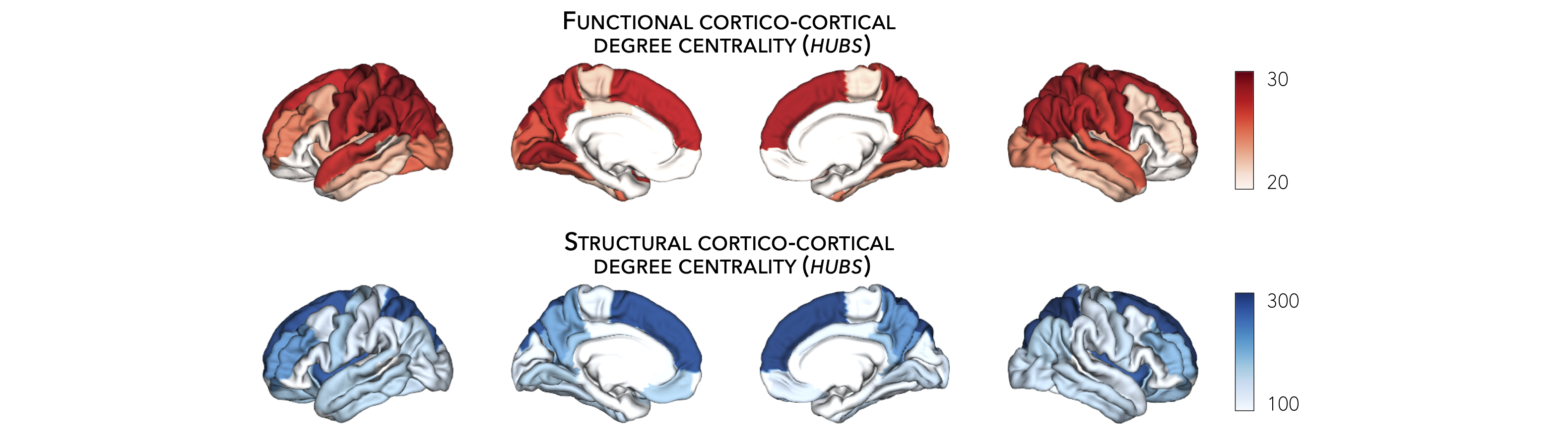
Cortical hubs
Normative structural and functional connectomes hold valuable information for relating macroscopic brain network organization to patterns of disease-related atrophy. Using the HCP connectivity data, we can first compute weighted (optimal for unthresholded connectivity matrices) degree centrality to identify structural and functional hub regions (i.e., brain regions with many connections). This is done by simply computing the sum of all weighted cortico-cortical connections for every region. Higher degree centrality denotes increased hubness.
Prerequisites
↪ Load cortico-cortical connectivity matrices
>>> import numpy as np
>>> from enigmatoolbox.plotting import plot_cortical
>>> from enigmatoolbox.utils.parcellation import parcel_to_surface

>>> # Compute weighted degree centrality measures from the connectivity data
>>> fc_ctx_dc = np.sum(fc_ctx, axis=0)
>>> sc_ctx_dc = np.sum(sc_ctx, axis=0)

>>> # Map parcellated data to the surface
>>> fc_ctx_dc_fsa5 = parcel_to_surface(fc_ctx_dc, 'aparc_fsa5')
>>> sc_ctx_dc_fsa5 = parcel_to_surface(sc_ctx_dc, 'aparc_fsa5')

>>> # Project the results on the surface brain
>>> plot_cortical(array_name=fc_ctx_dc_fsa5, surface_name="fsa5", size=(800, 400),
...               cmap='Reds', color_bar=True, color_range=(20, 30))

>>> plot_cortical(array_name=sc_ctx_dc_fsa5, surface_name="fsa5", size=(800, 400),
...               cmap='Blues', color_bar=True, color_range=(100, 300))
% Compute weighted degree centrality measures from the connectivity data
fc_ctx_dc           = sum(fc_ctx);
sc_ctx_dc           = sum(sc_ctx);

% Map parcellated data to the surface
fc_ctx_dc_fsa5      = parcel_to_surface(fc_ctx_dc, 'aparc_fsa5');
sc_ctx_dc_fsa5      = parcel_to_surface(sc_ctx_dc, 'aparc_fsa5');

% Project the results on the surface brain
f = figure,
  plot_cortical(fc_ctx_dc_fsa5, 'surface_name', 'fsa5', 'color_range', [20 30], ...
                'cmap', 'Reds', 'label_text', 'Functional degree centrality')

f = figure,
  plot_cortical(sc_ctx_dc_fsa5, 'surface_name', 'fsa5', 'color_range', [100 300], ...
                'cmap', 'Blues', 'label_text', 'Structural degree centrality')
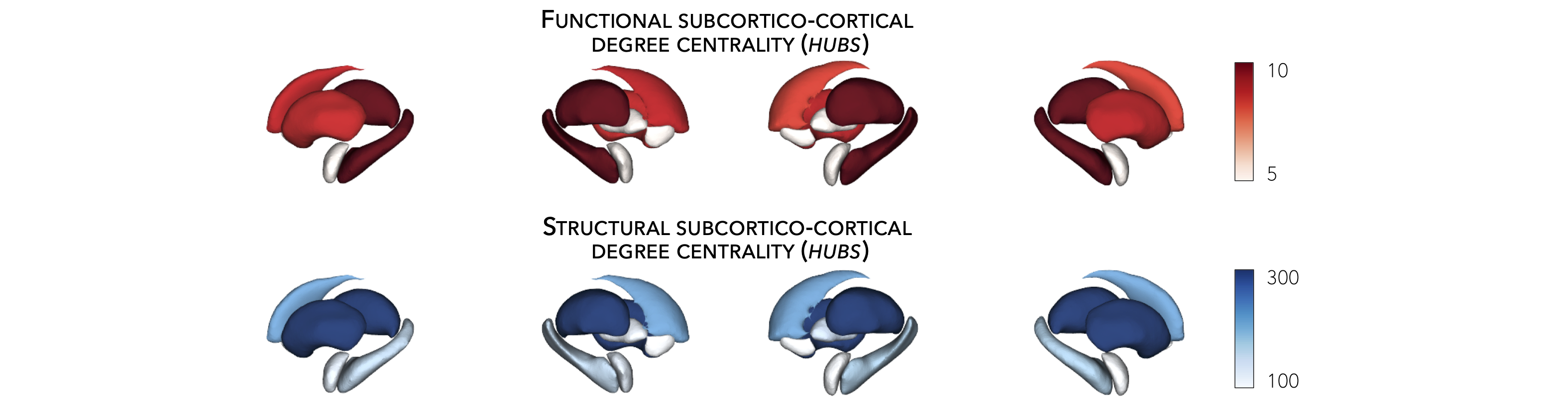
Subcortical hubs
The HCP connectivity data can also be used to identify structural and functional subcortico-cortical hub regions. As above, we simply compute the sum of all weighted subcortico-cortical connections for every subcortical area. Once again, higher degree centrality denotes increased hubness.
No ventricles, no problem 👌🏼
Because we do not have connectivity values for the ventricles, do make sure to set
the “ventricles” flag to False when displaying the findings on the subcortical surfaces.
Prerequisites
↪ Load subcortico-cortical connectivity matrices
>>> import numpy as np
>>> from enigmatoolbox.plotting import plot_subcortical

>>> # Compute weighted degree centrality measures from the connectivity data
>>> fc_sctx_dc = np.sum(fc_sctx, axis=1)
>>> sc_sctx_dc = np.sum(sc_sctx, axis=1)

>>> # Project the results on the surface brain
>>> plot_subcortical(array_name=fc_sctx_dc, ventricles=False, size=(800, 400),
...                  cmap='Reds', color_bar=True, color_range=(5, 10))

>>> plot_subcortical(array_name=sc_sctx_dc, ventricles=False, size=(800, 400),
...                  cmap='Blues', color_bar=True, color_range=(100, 300))
% Compute weighted degree centrality measures from the connectivity data
fc_sctx_dc          = sum(fc_sctx, 2);
sc_sctx_dc          = sum(sc_sctx, 2);

% Project the results on the surface brain
f = figure,
  plot_subcortical(fc_sctx_dc, 'ventricles', 'False', 'color_range', [5 10], ...
                   'cmap', 'Reds', 'label_text', 'Functional degree centrality')

f = figure,
  plot_subcortical(sc_sctx_dc, 'ventricles', 'False', 'color_range', [100 300], ...
                   'cmap', 'Blues', 'label_text', 'Structural degree centrality')
Hub-atrophy correlations
Now that we have established the spatial distribution of hubs in the brain, we can then assess whether these hub regions are selectively vulnerable to syndrome-specific atrophy patterns. For simplicity, in the following example, we will spatially correlate degree centrality measures to measures of cortical and subcortical atrophy (where lower values indicate greater atrophy relative to controls).
Prerequisites
↪ Load summary statistics or example data
↪ Re-order subcortical data (mega only)
↪ Z-score data (mega only)
↪ Load cortico-cortical and subcortico-cortical connectivity matrices
↪ Compute cortical-cortical and subcortico-cortical degree centrality
>>> import numpy as np

>>> # Remove subcortical values corresponding to the ventricles
>>> # (as we don't have connectivity values for them!)
>>> SV_d_noVent = SV_d.drop([np.where(SV['Structure'] == 'LLatVent')[0][0],
...                         np.where(SV['Structure'] == 'RLatVent')[0][0]]).reset_index(drop=True)

>>> # Perform spatial correlations between functional hubs and Cohen's d
>>> fc_ctx_r = np.corrcoef(fc_ctx_dc, CT_d)[0, 1]
>>> fc_sctx_r = np.corrcoef(fc_sctx_dc, SV_d_noVent)[0, 1]

>>> # Perform spatial correlations between structural hubs and Cohen's d
>>> sc_ctx_r = np.corrcoef(sc_ctx_dc, CT_d)[0, 1]
>>> sc_sctx_r = np.corrcoef(sc_sctx_dc, SV_d_noVent)[0, 1]

>>> # Store correlation coefficients
>>> rvals = {'functional cortical hubs': fc_ctx_r, 'functional subcortical hubs': fc_sctx_r,
...          'structural cortical hubs': sc_ctx_r, 'structural subcortical hubs': sc_sctx_r}
% Remove subcortical values corresponding the ventricles
% (as we don't have connectivity values for them!)
SV_d_noVent = SV_d;
SV_d_noVent([find(strcmp(SV.Structure, 'LLatVent')); ...
            find(strcmp(SV.Structure, 'RLatVent'))], :) = [];

% Perform spatial correlations between cortical hubs and Cohen's d
fc_ctx_r = corrcoef(fc_ctx_dc, CT_d);
sc_ctx_r = corrcoef(sc_ctx_dc, CT_d);

% Perform spatial correlations between structural hubs and Cohen's d
fc_sctx_r = corrcoef(fc_sctx_dc, SV_d_noVent);
sc_sctx_r = corrcoef(sc_sctx_dc, SV_d_noVent);

% Store correlation coefficients
rvals = cell2struct({fc_ctx_r(1, 2), fc_sctx_r(1, 2), sc_ctx_r(1, 2), sc_sctx_r(1, 2)}, ...
                    {'functional_cortical_hubs', 'functional_subcortical_hubs', ...
                     'structural_cortical_hubs', 'structural_subcortical_hubs'}, 2);
>>> import numpy as np

>>> # Remove subcortical values corresponding to the ventricles
>>> # (as we don't have connectivity values for them!)
>>> SV_z_mean_noVent = SV_z_mean.drop(['LLatVent', 'RLatVent']).reset_index(drop=True)

>>> # Perform spatial correlations between functional hubs and z-scores
>>> fc_ctx_r = np.corrcoef(fc_ctx_dc, CT_z_mean)[0, 1]
>>> fc_sctx_r = np.corrcoef(fc_sctx_dc, SV_z_mean_noVent)[0, 1]

>>> # Perform spatial correlations between structural hubs and z-scores
>>> sc_ctx_r = np.corrcoef(sc_ctx_dc, CT_z_mean)[0, 1]
>>> sc_sctx_r = np.corrcoef(sc_sctx_dc, SV_z_mean_noVent)[0, 1]

>>> # Store correlation coefficients
>>> rvals = {'functional cortical hubs': fc_ctx_r, 'functional subcortical hubs': fc_sctx_r,
...          'structural cortical hubs': sc_ctx_r, 'structural subcortical hubs': sc_sctx_r}
% Remove subcortical values corresponding the ventricles
% (as we don't have connectivity values for them!)
SV_z_mean_noVent = SV_z_mean;
SV_z_mean_noVent.LLatVent = [];
SV_z_mean_noVent.RLatVent = [];

% Perform spatial correlations between cortical hubs and Cohen's d
fc_ctx_r = corrcoef(fc_ctx_dc, CT_z_mean{:, :});
sc_ctx_r = corrcoef(sc_ctx_dc, CT_z_mean{:, :});

% Perform spatial correlations between structural hubs and Cohen's d
fc_sctx_r = corrcoef(fc_sctx_dc, SV_z_mean_noVent{:, :});
sc_sctx_r = corrcoef(sc_sctx_dc, SV_z_mean_noVent{:, :});

% Store correlation coefficients
rvals = cell2struct({fc_ctx_r(1, 2), fc_sctx_r(1, 2), sc_ctx_r(1, 2), sc_sctx_r(1, 2)}, ...
                    {'functional_cortical_hubs', 'functional_subcortical_hubs', ...
                     'structural_cortical_hubs', 'structural_subcortical_hubs'}, 2);
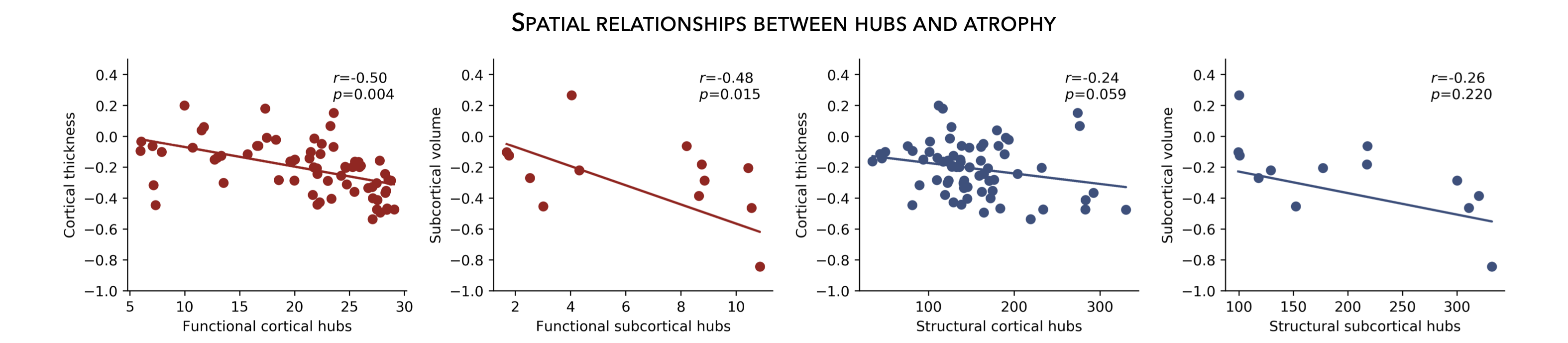
Plot hub-atrophy correlations
Now that we have done all the necessary analyses, we can finally display our correlations. Here, a negative correlation indicates that greater atrophy correlates with the spatial distribution of hub regions (greater degree centrality).
Prerequisites
     The script below can be used to show relationships between any two variables, as for example:
     degree centrality vs. atrophy
          ↪ Load summary statistics or example data
          ↪ Re-order subcortical data (mega only)
          ↪ Z-score data (mega only)
          ↪ Load cortico-cortical and subcortico-cortical connectivity matrices
          ↪ Compute cortical-cortical and subcortico-cortical degree centrality
          ↪ Assess statistical significance via spin permutation tests
>>> import matplotlib.pyplot as plt
>>> import numpy as np

>>> # Store degree centrality and atrophy measures
>>> meas = {('functional cortical hubs', 'cortical thickness'): [fc_ctx_dc, CT_d],
...         ('functional subcortical hubs', 'subcortical volume'): [fc_sctx_dc, SV_d_noVent],
...         ('structural cortical hubs', 'cortical thickness'): [sc_ctx_dc, CT_d],
...         ('structural subcortical hubs', 'subcortical volume'): [sc_sctx_dc, SV_d_noVent]}

>>> fig, axs = plt.subplots(1, 4, figsize=(15, 3))

>>> for k, (fn, dd) in enumerate(meas.items()):
>>>     # Define scatter colors
>>>     if k <= 1:
>>>         col = '#A8221C'
>>>     else:
>>>         col = '#324F7D'

>>>     # Plot relationships between hubs and atrophy
>>>     axs[k].scatter(meas[fn][0], meas[fn][1], color=col,
...                    label='$r$={:.2f}'.format(rvals[fn[0]]) + '\n$p$={:.3f}'.format(p_and_d[fn[0]][0]))
>>>     m, b = np.polyfit(meas[fn][0], meas[fn][1], 1)
>>>     axs[k].plot(meas[fn][0], m * meas[fn][0] + b, color=col)
>>>     axs[k].set_ylim((-1, 0.5))
>>>     axs[k].set_xlabel('{}'.format(fn[0].capitalize()))
>>>     axs[k].set_ylabel('{}'.format(fn[1].capitalize()))
>>>     axs[k].spines['top'].set_visible(False)
>>>     axs[k].spines['right'].set_visible(False)
>>>     axs[k].legend(loc=1, frameon=False, markerscale=0)

>>> fig.tight_layout()
>>> plt.show()
% Store degree centrality measures
meas  =  cell2struct({fc_ctx_dc.', fc_sctx_dc, sc_ctx_dc.', sc_sctx_dc}, ...
                     {'Functional_cortical_hubs', 'Functional_subcortical_hubs', ...
                     'Structural_cortical_hubs', 'Structural_subcortical_hubs'}, 2);
fns   = fieldnames(meas);

% Store atrophy measures
meas2 =  cell2struct({CT_d, SV_d_noVent}, {'Cortical_thickness', 'Subcortical_volume'}, 2);
fns2  = fieldnames(meas2);

f = figure,
    set(gcf,'color','w');
    set(gcf,'units','normalized','position',[0 0 1 0.3])
    k2 = [1 2 1 2];

    for k = 1:numel(fieldnames(meas))
        j = k2(k);

        % Define plot colors
        if k <= 2; col = [0.66 0.13 0.11]; else; col = [0.2 0.33 0.49]; end

        % Plot relationships between hubs and atrophy
        axs = subplot(1, 4, k); hold on
        s   = scatter(meas.(fns{k}), meas2.(fns2{j}), 88, col, 'filled');
        P1      = polyfit(meas.(fns{k}), meas2.(fns2{j}), 1);
        yfit_1  = P1(1) * meas.(fns{k}) + P1(2);
        plot(meas.(fns{k}), yfit_1, 'color',col, 'LineWidth', 3)
        ylim([-1 0.5])
        xlabel(strrep(fns{k}, '_', ' '))
        ylabel(strrep(fns2{j}, '_', ' '))
        legend(s, ['{\it r}=' num2str(round(rvals.(lower(fns{k})), 2)) newline ...
                  '{\it p}=' num2str(round(p_and_d.(lower(fns{k}))(1), 3))])
        legend boxoff
    end
>>> import matplotlib.pyplot as plt
>>> import numpy as np

>>> # Store degree centrality and atrophy measures
>>> meas = {('functional cortical hubs', 'cortical thickness'): [fc_ctx_dc, CT_z_mean],
...         ('functional subcortical hubs', 'subcortical volume'): [fc_sctx_dc, SV_z_mean_noVent],
...         ('structural cortical hubs', 'cortical thickness'): [sc_ctx_dc, CT_z_mean],
...         ('structural subcortical hubs', 'subcortical volume'): [sc_sctx_dc, SV_z_mean_noVent]}

>>> fig, axs = plt.subplots(1, 4, figsize=(15, 3))

>>> for k, (fn, dd) in enumerate(meas.items()):
>>>     # Define scatter colors
>>>     if k <= 1:
>>>         col = '#A8221C'
>>>     else:
>>>         col = '#324F7D'

>>>     # Plot relationships between hubs and atrophy
>>>     axs[k].scatter(meas[fn][0], meas[fn][1], color=col,
...                    label='$r$={:.2f}'.format(rvals[fn[0]]) + '\n$p$={:.3f}'.format(p_and_d[fn[0]][0]))
>>>     m, b = np.polyfit(meas[fn][0], meas[fn][1], 1)
>>>     axs[k].plot(meas[fn][0], m * meas[fn][0] + b, color=col)
>>>     axs[k].set_ylim((-3.5, 1.5))
>>>     axs[k].set_xlabel('{}'.format(fn[0].capitalize()))
>>>     axs[k].set_ylabel('{}'.format(fn[1].capitalize()))
>>>     axs[k].spines['top'].set_visible(False)
>>>     axs[k].spines['right'].set_visible(False)
>>>     axs[k].legend(loc=1, frameon=False, markerscale=0)

>>> fig.tight_layout()
>>> plt.show()
% Store degree centrality measures
meas  =  cell2struct({fc_ctx_dc, fc_sctx_dc.', sc_ctx_dc, sc_sctx_dc.'}, ...
                     {'Functional_cortical_hubs', 'Functional_subcortical_hubs', ...
             'Structural_cortical_hubs', 'Structural_subcortical_hubs'}, 2);
fns   = fieldnames(meas);

% Store atrophy measures
meas2 =  cell2struct({CT_z_mean{:, :}, SV_z_mean_noVent{:, :}}, ...
                     {'Cortical_thickness', 'Subcortical_volume'}, 2);
fns2  = fieldnames(meas2);

f = figure,
    set(gcf,'color','w');
    set(gcf,'units','normalized','position',[0 0 1 0.3])
    k2 = [1 2 1 2];

    for k = 1:numel(fieldnames(meas))
        j = k2(k);

        % Define plot colors
        if k <= 2; col = [0.66 0.13 0.11]; else; col = [0.2 0.33 0.49]; end

        % Plot relationships between hubs and atrophy
        axs = subplot(1, 4, k); hold on
        s   = scatter(meas.(fns{k}), meas2.(fns2{j}), 88, col, 'filled');
        P1      = polyfit(meas.(fns{k}), meas2.(fns2{j}), 1);
        yfit_1  = P1(1) * meas.(fns{k}) + P1(2);
        plot(meas.(fns{k}), yfit_1, 'color',col, 'LineWidth', 3)
        ylim([-3 1.5])
        xlabel(strrep(fns{k}, '_', ' '))
        ylabel(strrep(fns2{j}, '_', ' '))
        legend(s, ['{\it r}=' num2str(round(rvals.(lower(fns{k})), 2)) newline ...
                  '{\it p}=' num2str(round(p_and_d.(lower(fns{k}))(1), 3))])
        legend boxoff
    end