Spin permutation tests
This page contains descriptions and examples to assess statistical significance of two spatial maps.
Assess statistical significance
The intrinsic spatial smoothness in two given cortical maps may inflate the significance of their spatial correlation. To overcome this challenge, we assess statistical significance using spin permutation tests, a framework proposed by Alexander-Bloch and colleagues. To do so, we generate null models of overlap between cortical maps by projecting the spatial coordinates of cortical data onto the surface spheres, apply randomly sampled rotations, and reassign cortical values. We then compare the original correlation coefficients against the empirical distribution determined by the ensemble of spatially permuted correlation coefficients.
Prerequisites
Two brain maps from which you want to assess the signifcance of their correlations, as for example:
degree centrality vs. atrophy
     ↪ Load summary statistics or example data
     ↪ Re-order subcortical data (mega only)
     ↪ Z-score data (mega only)
     ↪ Load cortico-cortical and subcortico-cortical connectivity matrices
     ↪ Compute cortical-cortical and subcortico-cortical degree centrality
>>> from enigmatoolbox.permutation_testing import spin_test, shuf_test

>>> # Remove subcortical values corresponding to the ventricles
>>> # (as we don't have connectivity values for them!)
>>> SV_d_noVent = SV_d.drop([np.where(SV['Structure'] == 'LLatVent')[0][0],
...                         np.where(SV['Structure'] == 'RLatVent')[0][0]]).reset_index(drop=True)

>>> # Spin permutation testing for two cortical maps
>>> fc_ctx_p, fc_ctx_d = spin_test(fc_ctx_dc, CT_d, surface_name='fsa5', parcellation_name='aparc',
...                                type='pearson', n_rot=1000, null_dist=True)
>>> sc_ctx_p, sc_ctx_d = spin_test(sc_ctx_dc, CT_d, surface_name='fsa5', parcellation_name='aparc',
...                                type='pearson', n_rot=1000, null_dist=True)

>>> # Shuf permutation testing for two subcortical maps
>>> fc_sctx_p, fc_sctx_d = shuf_test(fc_sctx_dc, SV_d_noVent, n_rot=1000,
...                                  type='pearson', null_dist=True)
>>> sc_sctx_p, sc_sctx_d = shuf_test(sc_sctx_dc, SV_d_noVent, n_rot=1000,
...                                  type='pearson', null_dist=True)

>>> # Store p-values and null distributions
>>> p_and_d = {'functional cortical hubs': [fc_ctx_p, fc_ctx_d], 'functional subcortical hubs': [fc_sctx_p, fc_sctx_d],
...            'structural cortical hubs': [sc_ctx_p, sc_ctx_d], 'structural subcortical hubs': [sc_sctx_p, sc_sctx_d]}
% Remove subcortical values corresponding to the ventricles
% (as we don't have connectivity values for them!)
SV_d_noVent = SV_d;
SV_d_noVent([find(strcmp(SV.Structure, 'LLatVent')); ...
            find(strcmp(SV.Structure, 'RLatVent'))], :) = [];

% Spin permutation testing for two cortical maps
[fc_ctx_p, fc_ctx_d]   = spin_test(fc_ctx_dc, CT_d, 'surface_name', 'fsa5', ...
                                   'parcellation_name', 'aparc', 'n_rot', 1000, ...
                                   'type', 'pearson');
[sc_ctx_p, sc_ctx_d]   = spin_test(sc_ctx_dc, CT_d, 'surface_name', 'fsa5', ...
                                   'parcellation_name', 'aparc', 'n_rot', 1000, ...
                                   'type', 'pearson');

% Shuf permutation testing for two subcortical maps
[fc_sctx_p, fc_sctx_d] = shuf_test(fc_sctx_dc, SV_d_noVent, ...
                                   'n_rot', 1000, 'type', 'pearson');
[sc_sctx_p, sc_sctx_d] = shuf_test(sc_sctx_dc, SV_d_noVent, ...
                                   'n_rot', 1000, 'type', 'pearson');

% Store p-values and null distributions
p_and_d =  cell2struct({[fc_ctx_p; fc_ctx_d], [fc_sctx_p; fc_sctx_d], [sc_ctx_p; sc_ctx_d], [sc_sctx_p; sc_sctx_d]}, ...
                       {'functional_cortical_hubs', 'functional_subcortical_hubs', ...
                        'structural_cortical_hubs', 'structural_subcortical_hubs'}, 2);
>>> from enigmatoolbox.permutation_testing import spin_test, shuf_test

>>> # Remove subcortical values corresponding to the ventricles
>>> # (as we don't have connectivity values for them!)
>>> SV_z_mean_noVent = SV_z_mean.drop(['LLatVent', 'RLatVent']).reset_index(drop=True)

>>> # Spin permutation testing for two cortical maps
>>> fc_ctx_p, fc_ctx_d = spin_test(fc_ctx_dc, CT_z_mean, surface_name='fsa5', parcellation_name='aparc',
...                                type='pearson', n_rot=1000, null_dist=True)
>>> sc_ctx_p, sc_ctx_d = spin_test(sc_ctx_dc, CT_z_mean, surface_name='fsa5', parcellation_name='aparc',
...                                type='pearson', n_rot=1000, null_dist=True)

>>> # Shuf permutation testing for two subcortical maps
>>> fc_sctx_p, fc_sctx_d = shuf_test(fc_sctx_dc, SV_z_mean_noVent, n_rot=1000,
...                                  type='pearson', null_dist=True)
>>> sc_sctx_p, sc_sctx_d = shuf_test(sc_sctx_dc, SV_z_mean_noVent, n_rot=1000,
...                                  type='pearson', null_dist=True)

>>> # Store p-values and null distributions
>>> p_and_d = {'functional cortical hubs': [fc_ctx_p, fc_ctx_d], 'functional subcortical hubs': [fc_sctx_p, fc_sctx_d],
...            'structural cortical hubs': [sc_ctx_p, sc_ctx_d], 'structural subcortical hubs': [sc_sctx_p, sc_sctx_d]}
% Remove subcortical values corresponding to the ventricles
% (as we don't have connectivity values for them!)
SV_z_mean_noVent = SV_z_mean;
SV_z_mean_noVent.LLatVent = [];
SV_z_mean_noVent.RLatVent = [];

% Spin permutation testing for two cortical maps
[fc_ctx_p, fc_ctx_d]   = spin_test(fc_ctx_dc, CT_z_mean{:, :}, 'surface_name', ...
                                   'fsa5', 'parcellation_name', 'aparc', 'n_rot', ...
                                   1000, 'type', 'pearson');
[sc_ctx_p, sc_ctx_d]   = spin_test(sc_ctx_dc, CT_z_mean{:, :}, 'surface_name', ...
                                   'fsa5', 'parcellation_name', 'aparc', 'n_rot', ...
                                   1000, 'type', 'pearson');

% Shuf permutation testing for two subcortical maps
[fc_sctx_p, fc_sctx_d] = shuf_test(fc_sctx_dc, SV_z_mean_noVent{:, :}, ...
                                   'n_rot', 1000, 'type', 'pearson');
[sc_sctx_p, sc_sctx_d] = shuf_test(sc_sctx_dc, SV_z_mean_noVent{:, :}, ...
                                   'n_rot', 1000, 'type', 'pearson');

% Store p-values and null distributions
p_and_d =  cell2struct({[fc_ctx_p; fc_ctx_d], [fc_sctx_p; fc_sctx_d], [sc_ctx_p; sc_ctx_d], [sc_sctx_p; sc_sctx_d]}, ...
                       {'functional_cortical_hubs', 'functional_subcortical_hubs', ...
                        'structural_cortical_hubs', 'structural_subcortical_hubs'}, 2);
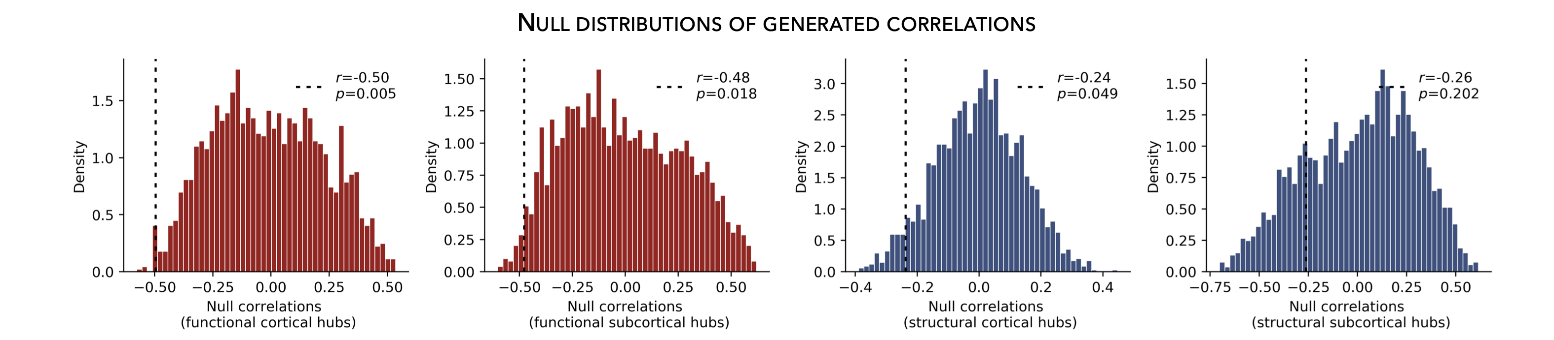
Plot null distributions
To better interpret statistical significance, we can plot the null distribution of generated correlations (i.e., “spun” or “shuffled” correlations) and overlay the correlation coefficient obtained from the empirical (i.e., real) brain maps.
>>> import matplotlib.pyplot as plt

>>> fig, axs = plt.subplots(1, 4, figsize=(15, 3))

>>> for k, (fn, dd) in enumerate(p_and_d.items()):
>>>     # Define plot colors
>>>     if k <= 1:
>>>         col = '#A8221C'     # red for functional hubs
>>>     else:
>>>         col = '#324F7D'     # blue for structural hubs

>>>     # Plot null distributions
>>>     axs[k].hist(dd[1], bins=50, density=True, color=col, edgecolor='white', lw=0.5)
>>>     axs[k].axvline(rvals[fn], lw=1.5, ls='--', color='k', dashes=(2, 3),
...                    label='$r$={:.2f}'.format(rvals[fn]) + '\n$p$={:.3f}'.format(dd[0]))
>>>     axs[k].set_xlabel('Null correlations \n ({})'.format(fn))
>>>     axs[k].set_ylabel('Density')
>>>     axs[k].spines['top'].set_visible(False)
>>>     axs[k].spines['right'].set_visible(False)
>>>     axs[k].legend(loc=1, frameon=False)

>>> fig.tight_layout()
>>> plt.show()
f = figure,
    set(gcf,'color','w');
    set(gcf,'units','normalized','position',[0 0 1 0.3])
    fns = fieldnames(p_and_d);

    for k = 1:numel(fieldnames(rvals))
        % Define plot colors
        if k <= 2; col = [0.66 0.13 0.11]; else; col = [0.2 0.33 0.49]; end

        % Plot null distributions
        axs = subplot(1, 4, k); hold on
        h = histogram(p_and_d.(fns{k})(2:end), 50, 'Normalization', 'pdf', 'edgecolor', 'w', ...
                      'facecolor', col, 'facealpha', 1, 'linewidth', 0.5);
        l = line([rvals.(fns{k}) rvals.(fns{k})], get(gca, 'ylim'), 'linestyle', '--', ...
                 'color', 'k', 'linewidth', 1.5);
        xlabel(['Null correlations' newline '(' strrep(fns{k}, '_', ' ') ')'])
        ylabel('Density')
        legend(l,['{\it r}=' num2str(round(rvals.(fns{k}), 2)) newline ...
                  '{\it p}=' num2str(round(p_and_d.(fns{k})(1), 3))])
        legend boxoff
    end