Cross-disorder effect¶

This page contains descriptions and examples to perform cross-disorder analyses to explore brain structural abnormalities that are common or different across disorders.

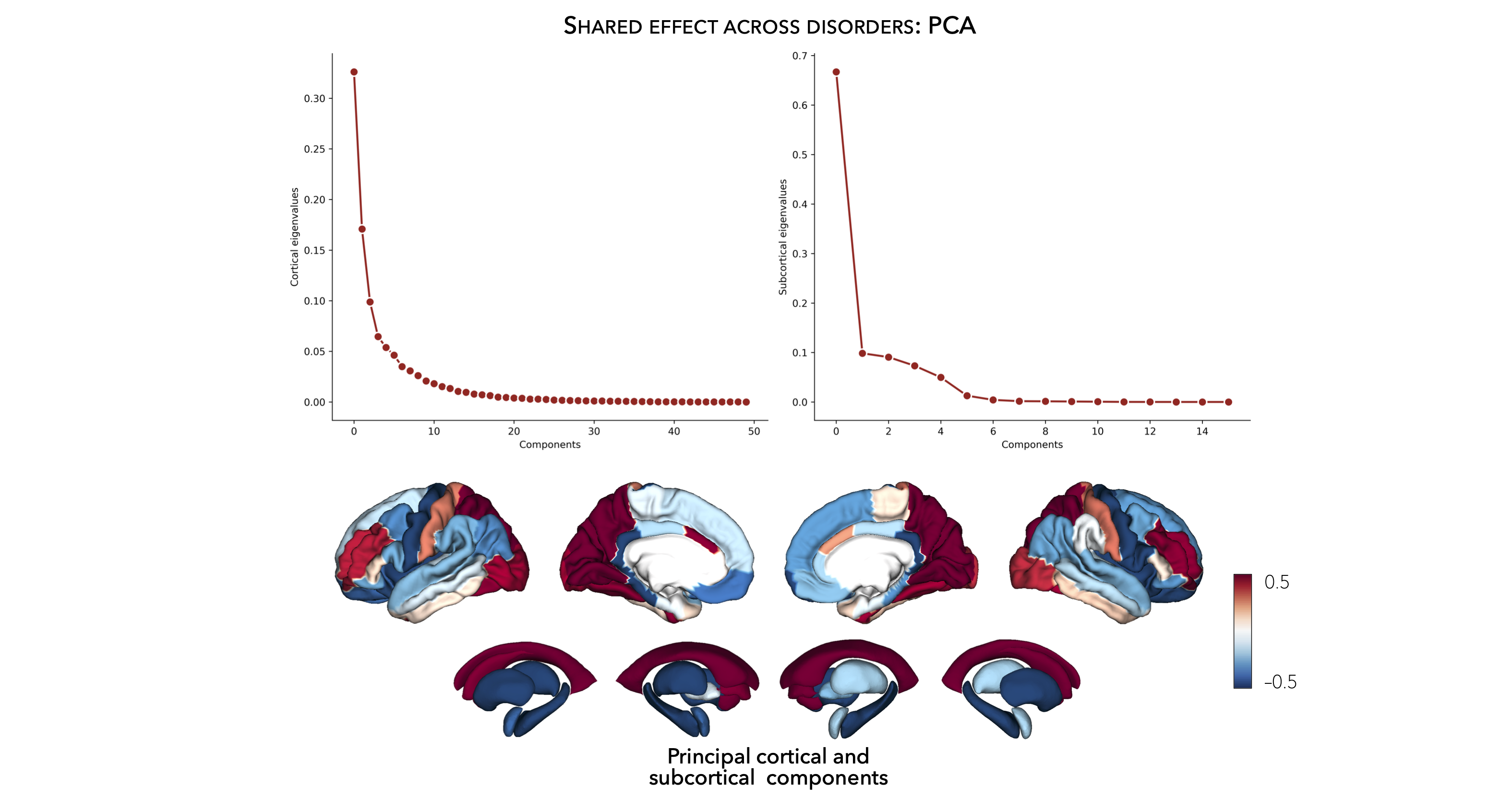
Principal component analysis¶

To yield novel insights into brain structural abnormalities that are common or different across disorders, we can explore shared and disease-specific morphometric signatures by applying a principal component analysis (PCA) to any combination of disease-specific summary statistics (or other imported data), resulting in shared latent components that can be used for further analysis.

>>> from enigmatoolbox.cross_disorder import cross_disorder_effect
>>> from enigmatoolbox.plotting import plot_cortical, plot_subcortical
>>> from enigmatoolbox.utils import parcel_to_surface
>>> import matplotlib.pyplot as plt

>>> # Extract shared disorder effects
>>> components, variance, names = cross_disorder_effect()

>>> # Visualize cortical and subcortical eigenvalues in scree plots
>>> fig, ax = plt.subplots(1, 2, figsize=(14, 6))
>>> for ii, jj in enumerate(components):
>>>    ax[ii].plot(variance[jj], lw=2, color='#A8221C', zorder=1)
>>>    ax[ii].scatter(range(variance[jj].size), variance[jj], s=78, color='#A8221C',
>>>                   linewidth=1.5, edgecolor='w', zorder=3)
>>>    ax[ii].set_xlabel('Components')

>>>    if ii == 0:
>>>         ax[ii].set_ylabel('Cortical eigenvalues')
>>>    else:
>>>         ax[ii].set_ylabel('Subcortical eigenvalues')

>>>    ax[ii].spines['top'].set_visible(False)
>>>    ax[ii].spines['right'].set_visible(False)

>>> fig.tight_layout()
>>> plt.show()

>>> # Visualize the first cortical and subcortical components on the surface brains
>>> plot_cortical(parcel_to_surface(components['cortex'][:, 0], 'aparc_fsa5'), color_range=(-0.5, 0.5),
...               cmap='RdBu_r', color_bar=True, size=(800, 400))

>>> plot_subcortical(components['subcortex'][:, 0], color_range=(-0.5, 0.5),
...                  cmap='RdBu_r', color_bar=True, size=(800, 400))

% Extract shared disorder effects
[components, variance, ~, names] = cross_disorder_effect();

% Visualize cortical and subcortical eigenvalues in scree plots
fns  = fieldnames(components);

f = figure,
set(gcf,'color','w');
set(gcf,'units','normalized','position',[0 0 .75 0.3])

for ii = 1:numel(fieldnames(components))
     axs = subplot(1, 2, ii); hold on
     s = scatter(1:size(components.(fns{ii}), 2), variance.(fns{ii}), 128, [0.66 0.13 0.11], 'filled');
     s.LineWidth = 1.5; s.MarkerEdgeColor = 'w';

     plot(1:size(components.(fns{ii}), 2), variance.(fns{ii}), 'linewidth', 2, 'color', [0.66 0.13 0.11])
     xlabel('Components')

     if ii == 1
          ylabel('Cortical eigenvalues')
     else
          ylabel('Subcortical eigenvalues')
     end
end

% Visualize the first cortical and subcortical components on the surface brains
f = figure,
    plot_cortical(parcel_to_surface(components.cortex(:, 1)), 'color_range', [-0.5 0.5], 'cmap', 'RdBu_r')

f = figure,
    plot_subcortical(components.subcortex(:, 1), 'color_range', [-0.5 0.5], 'cmap', 'RdBu_r')

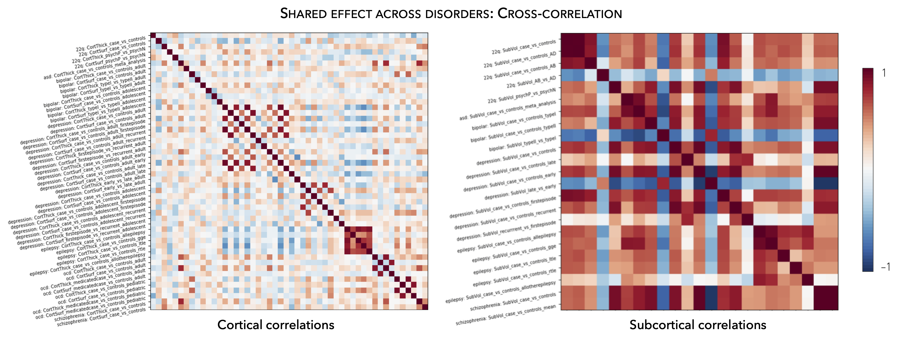
Cross-correlation¶

We can also explore shared and disease-specific morphometric signatures by systematically cross-correlating patterns of brain structural abnormalities with any combination of summary statistics (or other pre-loaded ENIGMA-type data), resulting in a correlation matrix

>>> from enigmatoolbox.cross_disorder import cross_disorder_effect
>>> from nilearn import plotting

>>> # Extract shared disorder effects
>>> correlation_matrix, names = cross_disorder_effect(method='correlation')

>>> # Plot correlation matrices
>>> plotting.plot_matrix(correlation_matrix['cortex'], figure=(12, 8), labels=names['cortex'], vmax=1,
...                      vmin=-1, cmap='RdBu_r', auto_fit=False)

>>> plotting.plot_matrix(correlation_matrix['subcortex'], figure=(12, 8), labels=names['subcortex'], vmax=1,
...                      vmin=-1, cmap='RdBu_r', auto_fit=False)

% Extract shared disorder effects
[~, ~, correlation_matrix, names] = cross_disorder_effect('method', 'correlation');

% Plot correlation matrices
f = figure('units','normalized','outerposition',[0 0 .65 1]),
    imagesc(correlation_matrix.cortex, [-1 1])
    axis square;
    colormap(RdBu_r);
    colorbar;
    set(gca, 'YTick', 1:1:size(correlation_matrix.cortex, 1), ...
        'YTickLabel', strrep(names.cortex, '_', ' '), 'XTick', 1:1:size(correlation_matrix.cortex, 1), ...
        'XTickLabel', strrep(names.cortex, '_', ' '), 'XTickLabelRotation', 45)

f = figure('units','normalized','outerposition',[0 0 .65 1]),
    imagesc(correlation_matrix.subcortex, [-1 1])
    axis square;
    colormap(RdBu_r);
    colorbar;
    set(gca, 'YTick', 1:1:size(correlation_matrix.subcortex, 1), ...
        'YTickLabel', strrep(names.subcortex, '_', ' '), 'XTick', 1:1:size(correlation_matrix.subcortex, 1), ...
        'XTickLabel', strrep(names.subcortex, '_', ' '), 'XTickLabelRotation', 45)