Epicenter mapping
This page contains descriptions and examples to identify disease epicenters. For additional details on disease epicenter mapping, please see our manuscript entitled Network-based atrophy modeling in the common epilepsies: a worldwide ENIGMA study.
Cortical epicenters
Using the HCP connectivity data, we can also identify epicenters of cortical atrophy. Disease epicenters are regions whose functional and/or structural connectivity profile spatially resembles a given disease-related atrophy map. Hence, disease epicenters can be identified by spatially correlating every region’s healthy functional and/or structural connectivity profiles (i.e., cortico-cortical connectivity) to whole-brain atrophy patterns in a given disease. This approach must be repeated systematically across the whole brain, assessing the statistical significance of the spatial similarity of every region’s functional and/or structural connectivity profiles to disease-specific abnormality maps with spatial permutation tests. Cortical and subcortical (see tutorial below) epicenter regions can then be identified if their connectivity profiles are significantly correlated with the disease-specific abnormality map. Regardless of its atrophy level, a cortical (or subcortical) region could potentially be an epicenter if it is (i) strongly connected to other high-atrophy regions and (ii) weakly connected to low-atrophy regions.
In this tutorial, our atrophy map was derived from cortical thickness decreases in individuals with left TLE.
Epicenters? 🤔
Cortical and subcortical epicenter regions are identified if their connectivity profiles correlate with a disease-specific cortical atrophy map. In the following examples, regions with strong negative correlations represent disease epicenters. Moreover, and regardless of its atrophy level, a cortical or subcortical region can be an epicenter if it is (i) strongly connected to other high-atrophy cortical regions and (ii) weakly connected to low-atrophy cortical regions.
Prerequisites
↪ Load summary statistics or example data
↪ Z-score data (mega only)
↪ Load cortico-cortical connectivity matrices
>>> import numpy as np
>>> from enigmatoolbox.permutation_testing import spin_test

>>> # Identify cortical epicenters (from functional connectivity)
>>> fc_ctx_epi = []
>>> fc_ctx_epi_p = []
>>> for seed in range(fc_ctx.shape[0]):
>>>     seed_con = fc_ctx[:, seed]
>>>     fc_ctx_epi = np.append(fc_ctx_epi, np.corrcoef(seed_con, CT_d)[0, 1])
>>>     fc_ctx_epi_p = np.append(fc_ctx_epi_p,
...                              spin_test(seed_con, CT_d, surface_name='fsa5', parcellation_name='aparc',
...                                        type='pearson', n_rot=1000, null_dist=False))

>>> # Identify cortical epicenters (from structural connectivity)
>>> sc_ctx_epi = []
>>> sc_ctx_epi_p = []
>>> for seed in range(sc_ctx.shape[0]):
>>>     seed_con = sc_ctx[:, seed]
>>>     sc_ctx_epi = np.append(sc_ctx_epi, np.corrcoef(seed_con, CT_d)[0, 1])
>>>     sc_ctx_epi_p = np.append(sc_ctx_epi_p,
...                              spin_test(seed_con, CT_d, surface_name='fsa5', parcellation_name='aparc',
...                                        type='pearson', n_rot=1000, null_dist=False))
% Identify cortical epicenter values (from functional connectivity)
fc_ctx_epi              = zeros(size(fc_ctx, 1), 1);
fc_ctx_epi_p            = zeros(size(fc_ctx, 1), 1);
for seed = 1:size(fc_ctx, 1)
    seed_conn           = fc_ctx(:, seed);
    r_tmp               = corrcoef(seed_conn, CT_d);
    fc_ctx_epi(seed)    = r_tmp(1, 2);
    fc_ctx_epi_p(seed)  = spin_test(seed_conn, CT_d, 'surface_name', 'fsa5', 'parcellation_name', ...
                                    'aparc', 'n_rot', 1000, 'type', 'pearson');
end

% Identify cortical epicenter values (from structural connectivity)
sc_ctx_epi              = zeros(size(sc_ctx, 1), 1);
sc_ctx_epi_p            = zeros(size(sc_ctx, 1), 1);
for seed = 1:size(sc_ctx, 1)
    seed_conn           = sc_ctx(:, seed);
    r_tmp               = corrcoef(seed_conn, CT_d);
    sc_ctx_epi(seed)    = r_tmp(1, 2);
    sc_ctx_epi_p(seed)  = spin_test(seed_conn, CT_d, 'surface_name', 'fsa5', 'parcellation_name', ...
                                    'aparc', 'n_rot', 1000, 'type', 'pearson');
end
>>> import numpy as np
>>> from enigmatoolbox.permutation_testing import spin_test

>>> # Identify cortical epicenters (from functional connectivity)
>>> fc_ctx_epi = []
>>> fc_ctx_epi_p = []
>>> for seed in range(fc_ctx.shape[0]):
>>>     seed_con = fc_ctx[:, seed]
>>>     fc_ctx_epi = np.append(fc_ctx_epi, np.corrcoef(seed_con, CT_z_mean)[0, 1])
>>>     fc_ctx_epi_p = np.append(fc_ctx_epi_p,
...                              spin_test(seed_con, CT_z_mean, surface_name='fsa5', parcellation_name='aparc',
...                                        type='pearson', n_rot=1000, null_dist=False))

>>> # Identify cortical epicenters (from structural connectivity)
>>> sc_ctx_epi = []
>>> sc_ctx_epi_p = []
>>> for seed in range(sc_ctx.shape[0]):
>>>     seed_con = sc_ctx[:, seed]
>>>     sc_ctx_epi = np.append(sc_ctx_epi, np.corrcoef(seed_con, CT_z_mean)[0, 1])
>>>     sc_ctx_epi_p = np.append(sc_ctx_epi_p,
...                              spin_test(seed_con, CT_z_mean, surface_name='fsa5', parcellation_name='aparc',
...                                        type='pearson', n_rot=1000, null_dist=False))
% Identify cortical epicenter values (from functional connectivity)
fc_ctx_epi              = zeros(size(fc_ctx, 1), 1);
fc_ctx_epi_p            = zeros(size(fc_ctx, 1), 1);
for seed = 1:size(fc_ctx, 1)
    seed_conn           = fc_ctx(:, seed);
    r_tmp               = corrcoef(seed_conn, CT_z_mean{:, :});
    fc_ctx_epi(seed)    = r_tmp(1, 2);
    fc_ctx_epi_p(seed)  = spin_test(seed_conn, CT_z_mean{:, :}, 'surface_name', 'fsa5', ...
                                    'parcellation_name', 'aparc', 'n_rot', 1000, 'type', 'pearson');
end

% Identify cortical epicenter values (from structural connectivity)
sc_ctx_epi              = zeros(size(sc_ctx, 1), 1);
sc_ctx_epi_p            = zeros(size(sc_ctx, 1), 1);
for seed = 1:size(sc_ctx, 1)
    seed_conn           = sc_ctx(:, seed);
    r_tmp               = corrcoef(seed_conn, CT_z_mean{:, :});
    sc_ctx_epi(seed)    = r_tmp(1, 2);
    sc_ctx_epi_p(seed)  = spin_test(seed_conn, CT_z_mean{:, :}, 'surface_name', 'fsa5', ...
                                    'parcellation_name', 'aparc', 'n_rot', 1000, 'type', 'pearson');
end
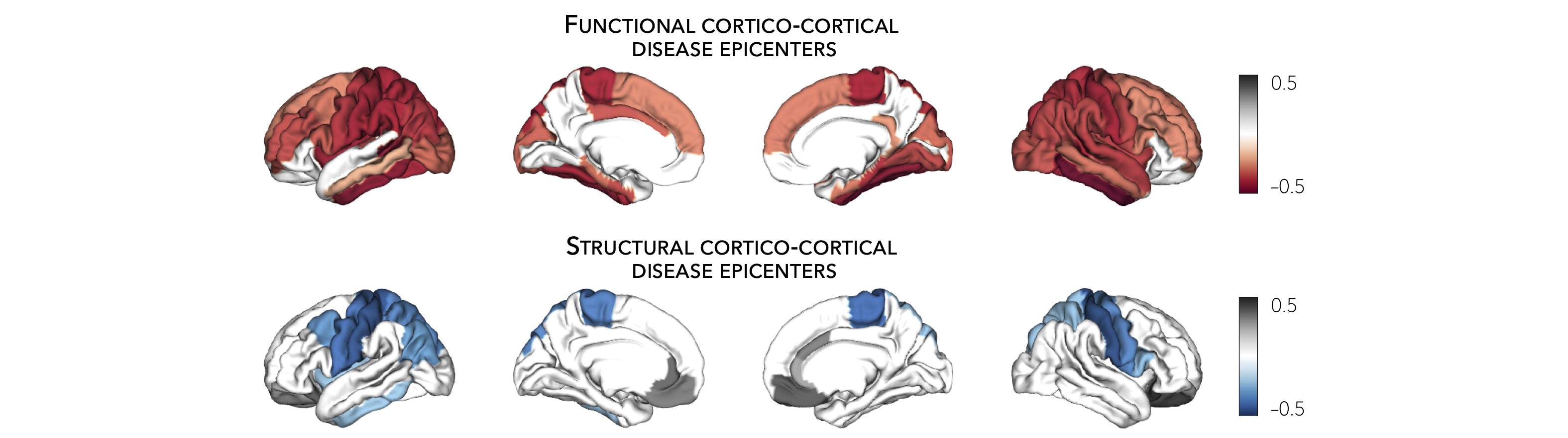
As we have assessed the significance of every spatial correlation between seed-based cortico-cortical connectivity and cortical atrophy measures using spin permutation tests, we can set a significance threshold to identify disease epicenters. In the following example, we set a lenient threshold of p < 0.1 (i.e., correlation coefficients were set to zeros for regions whose p-values were greater than 0.1). We are, thus, displaying only correlation coefficients whose significances passes at least these lenient thresholds.
>>> import numpy as np
>>> from enigmatoolbox.utils.parcellation import parcel_to_surface
>>> from enigmatoolbox.plotting import plot_cortical

>>> # Project the results on the surface brain
>>> # Selecting only regions with p < 0.1 (functional epicenters)
>>> fc_ctx_epi_p_sig = np.zeros_like(fc_ctx_epi_p)
>>> fc_ctx_epi_p_sig[np.argwhere(fc_ctx_epi_p < 0.1)] = fc_ctx_epi[np.argwhere(fc_ctx_epi_p < 0.1)]
>>> plot_cortical(array_name=parcel_to_surface(fc_ctx_epi_p_sig, 'aparc_fsa5'), surface_name="fsa5", size=(800, 400),
...               cmap='GyRd_r', color_bar=True, color_range=(-0.5, 0.5))

>>> # Selecting only regions with p < 0.1 (structural epicenters)
>>> sc_ctx_epi_p_sig = np.zeros_like(sc_ctx_epi_p)
>>> sc_ctx_epi_p_sig[np.argwhere(sc_ctx_epi_p < 0.1)] = sc_ctx_epi[np.argwhere(sc_ctx_epi_p < 0.1)]
>>> plot_cortical(array_name=parcel_to_surface(sc_ctx_epi_p_sig, 'aparc_fsa5'), surface_name="fsa5", size=(800, 400),
...               cmap='GyBu_r', color_bar=True, color_range=(-0.5, 0.5))
% Project the results on the surface brain
% Selecting only regions with p < 0.1 (functional epicenters)
fc_ctx_epi_p_sig = zeros(length(fc_ctx_epi_p), 1);
fc_ctx_epi_p_sig(find(fc_ctx_epi_p < 0.1)) = fc_ctx_epi(fc_ctx_epi_p<0.1);
f = figure,
    plot_cortical(parcel_to_surface(fc_ctx_epi_p_sig, 'aparc_fsa5'), ...
                'color_range', [-0.5 0.5], 'cmap', 'GyRd_r')

% Selecting only regions with p < 0.1 (structural epicenters)
sc_ctx_epi_p_sig = zeros(length(sc_ctx_epi_p), 1);
sc_ctx_epi_p_sig(find(sc_ctx_epi_p < 0.1)) = sc_ctx_epi(sc_ctx_epi_p<0.1);
f = figure,
    plot_cortical(parcel_to_surface(sc_ctx_epi_p_sig, 'aparc_fsa5'), ...
                'color_range', [-0.5 0.5], 'cmap', 'GyBu_r')
Subcortical epicenters
Similar to the cortical epicenter approach, we can identify subcortical epicenters of cortical atrophy by correlating every subcortical region’s seed-based connectivity profile (e.g., subcortico-cortical connectivity) with a whole-brain cortical atrophy map. As above, our atrophy map was derived from cortical thickness decreases in individuals with left TLE.
Prerequisites
↪ Load summary statistics or example data
↪ Z-score data (mega only)
↪ Load subcortico-cortical connectivity matrices
>>> import numpy as np
>>> from enigmatoolbox.permutation_testing import spin_test

>>> # Identify subcortical epicenters (from functional connectivity)
>>> fc_sctx_epi = []
>>> fc_sctx_epi_p = []
>>> for seed in range(fc_sctx.shape[0]):
>>>     seed_con = fc_sctx[seed, :]
>>>     fc_sctx_epi = np.append(fc_sctx_epi, np.corrcoef(seed_con, CT_d)[0, 1])
>>>     fc_sctx_epi_p = np.append(fc_sctx_epi_p,
...                               spin_test(seed_con, CT_d, surface_name='fsa5', n_rot=1000))

>>> # Identify subcortical epicenters (from structural connectivity)
>>> sc_sctx_epi = []
>>> sc_sctx_epi_p = []
>>> for seed in range(sc_sctx.shape[0]):
>>>     seed_con = sc_sctx[seed, :]
>>>     sc_sctx_epi = np.append(sc_sctx_epi, np.corrcoef(seed_con, CT_d)[0, 1])
>>>     sc_sctx_epi_p = np.append(sc_sctx_epi_p,
...                               spin_test(seed_con, CT_d, surface_name='fsa5', n_rot=1000))
% Identify subcortical epicenter values (from functional connectivity)
fc_sctx_epi             = zeros(size(fc_sctx, 1), 1);
fc_sctx_epi_p           = zeros(size(fc_sctx, 1), 1);
for seed = 1:size(fc_sctx, 1)
    seed_conn           = fc_sctx(seed, :);
    r_tmp               = corrcoef(seed_conn, CT_d);
    fc_sctx_epi(seed)   = r_tmp(1, 2);
    fc_sctx_epi_p(seed) = spin_test(seed_conn, CT_d, 'surface_name', 'fsa5', 'parcellation_name', ...
                                    'aparc', 'n_rot', 1000, 'type', 'pearson');
end

% Identify subcortical epicenter values (from structural connectivity)
sc_sctx_epi             = zeros(size(sc_sctx, 1), 1);
sc_sctx_epi_p           = zeros(size(sc_sctx, 1), 1);
for seed = 1:size(sc_sctx, 1)
    seed_conn           = sc_sctx(seed, :);
    r_tmp               = corrcoef(seed_conn, CT_d);
    sc_sctx_epi(seed)   = r_tmp(1, 2);
    sc_sctx_epi_p(seed) = spin_test(seed_conn, CT_d, 'surface_name', 'fsa5', 'parcellation_name', ...
                                    'aparc', 'n_rot', 1000, 'type', 'pearson');
end
>>> import numpy as np
>>> from enigmatoolbox.permutation_testing import spin_test

>>> # Identify subcortical epicenters (from functional connectivity)
>>> fc_sctx_epi = []
>>> fc_sctx_epi_p = []
>>> for seed in range(fc_sctx.shape[0]):
>>>     seed_con = fc_sctx[seed, :]
>>>     fc_sctx_epi = np.append(fc_sctx_epi, np.corrcoef(seed_con, CT_z_mean)[0, 1])
>>>     fc_sctx_epi_p = np.append(fc_sctx_epi_p,
...                               spin_test(seed_con, CT_z_mean, surface_name='fsa5', n_rot=1000))

>>> # Identify subcortical epicenters (from structural connectivity)
>>> sc_sctx_epi = []
>>> sc_sctx_epi_p = []
>>> for seed in range(sc_sctx.shape[0]):
>>>     seed_con = sc_sctx[seed, :]
>>>     sc_sctx_epi = np.append(sc_sctx_epi, np.corrcoef(seed_con, CT_z_mean)[0, 1])
>>>     sc_sctx_epi_p = np.append(sc_sctx_epi_p,
...                               spin_test(seed_con, CT_z_mean, surface_name='fsa5', n_rot=1000))
% Identify subcortical epicenter values (from functional connectivity)
fc_sctx_epi             = zeros(size(fc_sctx, 1), 1);
fc_sctx_epi_p           = zeros(size(fc_sctx, 1), 1);
for seed = 1:size(fc_sctx, 1)
    seed_conn           = fc_sctx(seed, :);
    r_tmp               = corrcoef(seed_conn, CT_z_mean{:, :});
    fc_sctx_epi(seed)   = r_tmp(1, 2);
    fc_sctx_epi_p(seed) = spin_test(seed_conn, CT_z_mean{:, :}, 'surface_name', 'fsa5', ...
                                    'parcellation_name', 'aparc', 'n_rot', 1000, 'type', 'pearson');
end

% Identify subcortical epicenter values (from structural connectivity)
sc_sctx_epi             = zeros(size(sc_sctx, 1), 1);
sc_sctx_epi_p           = zeros(size(sc_sctx, 1), 1);
for seed = 1:size(sc_sctx, 1)
    seed_conn           = sc_sctx(seed, :);
    r_tmp               = corrcoef(seed_conn, CT_z_mean{:, :});
    sc_sctx_epi(seed)   = r_tmp(1, 2);
    sc_sctx_epi_p(seed) = spin_test(seed_conn, CT_z_mean{:, :}, 'surface_name', 'fsa5', ...
                                    'parcellation_name', 'aparc', 'n_rot', 1000, 'type', 'pearson');
end
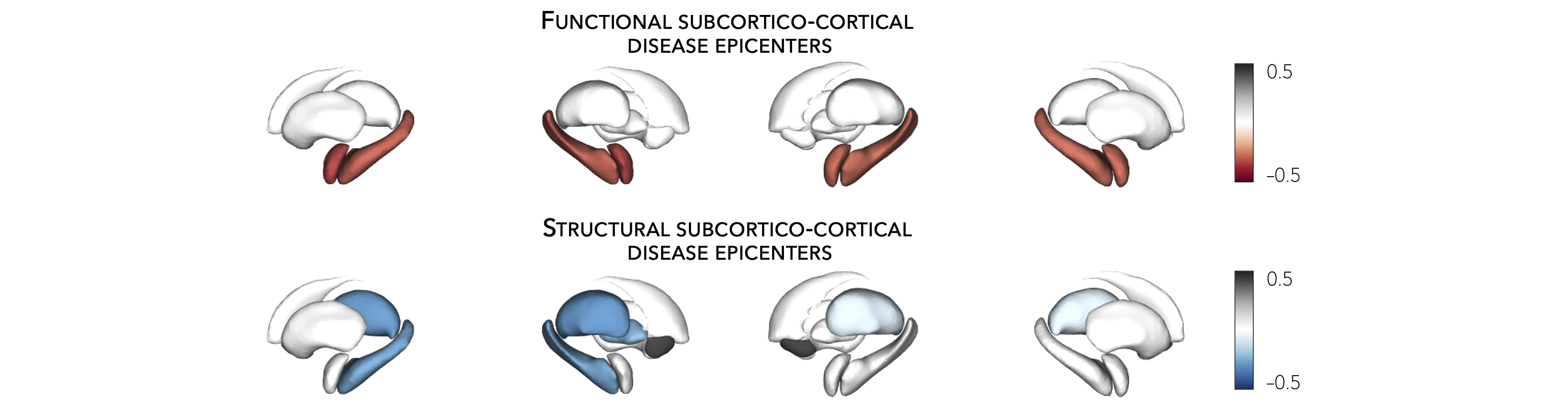
As in the cortical epicenters example above, we have assessed the significance of every spatial correlation between seed-based subcortico-cortical connectivity and cortical atrophy measures using spin permutation tests, and set a lenient threshold of p < 0.1 (i.e., correlation coefficients were set to zeros for regions whose p-values were greater than 0.1). We are, thus, displaying only correlation coefficients whose significances passes at least these lenient thresholds.
>>> import numpy as np
>>> from enigmatoolbox.plotting import plot_subcortical

>>> # Project the results on the surface brain
>>> # Selecting only regions with p < 0.1 (functional epicenters)
>>> fc_sctx_epi_p_sig = np.zeros_like(fc_sctx_epi_p)
>>> fc_sctx_epi_p_sig[np.argwhere(fc_sctx_epi_p < 0.1)] = fc_sctx_epi[np.argwhere(fc_sctx_epi_p < 0.1)]
>>> plot_subcortical(fc_sctx_epi_p_sig, ventricles=False, size=(800, 400),
...                  cmap='GyRd_r', color_bar=True, color_range=(-0.5, 0.5))

>>> # Selecting only regions with p < 0.1 (functional epicenters)
>>> sc_sctx_epi_p_sig = np.zeros_like(sc_sctx_epi_p)
>>> sc_sctx_epi_p_sig[np.argwhere(sc_sctx_epi_p < 0.1)] = sc_sctx_epi[np.argwhere(sc_sctx_epi_p < 0.1)]
>>> plot_subcortical(sc_sctx_epi_p_sig, ventricles=False, size=(800, 400),
...                  cmap='GyBu_r', color_bar=True, color_range=(-0.5, 0.5))
% Project the results on the surface brain
% Selecting only regions with p < 0.1 (functional epicenters)
fc_sctx_epi_p_sig = zeros(length(fc_sctx_epi_p), 1);
fc_sctx_epi_p_sig(find(fc_sctx_epi_p < 0.1)) = fc_sctx_epi(fc_sctx_epi_p<0.1);
f = figure,
    plot_subcortical(fc_sctx_epi_p_sig, 'ventricles', 'False', ...
                    'color_range', [-0.5 0.5], 'cmap', 'GyRd_r')

% Selecting only regions with p < 0.1 (structural epicenters)
sc_sctx_epi_p_sig = zeros(length(sc_sctx_epi_p), 1);
sc_sctx_epi_p_sig(find(sc_sctx_epi_p < 0.1)) = sc_sctx_epi(sc_sctx_epi_p<0.1);
f = figure,
    plot_subcortical(sc_sctx_epi_p_sig, 'ventricles', 'False', ...
                    'color_range', [-0.5 0.5], 'cmap', 'GyBu_r')